Grid Projection¶

A grid projection traces a regular 2D grid of rays through the mesh and integrates a field along each ray. This can be used to make images like column density maps.

Setting up¶

A grid projection requires four parameters:

extent – the spatial range of the grid in the image plane
npix – the number of pixels (square, or (nx, ny))
bounds – the integration limits along the line of sight
center – the rotation center; required for any projection other than the default 'xy' (or None for an xy projection)

Python

import numpy as np
import vortrace as vt

# Load your data
# pos: (N, 3), rho: (N,), vol: (N,)
BoxSize = 100.0
pc = vt.ProjectionCloud(
    pos, rho, vol=vol,
    boundbox=[0, BoxSize, 0, BoxSize, 0, BoxSize],
)

# Define the projection grid
L = 75.0
extent = [BoxSize / 2 - L / 2, BoxSize / 2 + L / 2]
bounds = [0, BoxSize]
npix = 256

# Project along z (default) -- center not required
image_xy = pc.grid_projection(extent, npix, bounds, center=None)

# Project along y (xz plane) -- center is required
center = [BoxSize / 2, BoxSize / 2, BoxSize / 2]
image_xz = pc.grid_projection(extent, npix, bounds, center, proj='xz')

C++

#include <vortrace/vortrace.hpp>
#include <vector>
#include <array>

// pos, fields, npart loaded from your data source
double BoxSize = 100.0;
std::array<double, 6> subbox = {0, BoxSize, 0, BoxSize, 0, BoxSize};

PointCloud cloud;
cloud.loadPoints(pos, npart, fields, npart, 1, subbox);
cloud.buildTree();

// Build a grid of rays along the z-axis
double L = 75.0;
size_t npix = 256;
double cx = BoxSize / 2, cy = BoxSize / 2;
double dx = L / npix;

std::vector<Float> starts(3 * npix * npix);
std::vector<Float> ends(3 * npix * npix);

for (size_t iy = 0; iy < npix; iy++) {
    for (size_t ix = 0; ix < npix; ix++) {
        size_t idx = 3 * (iy * npix + ix);
        double x = cx - L / 2 + (ix + 0.5) * dx;
        double y = cy - L / 2 + (iy + 0.5) * dx;
        starts[idx]     = x;  starts[idx+1] = y;  starts[idx+2] = 0.0;
        ends[idx]       = x;  ends[idx+1]   = y;  ends[idx+2]   = BoxSize;
    }
}

Projection proj(starts.data(), ends.data(), npix * npix);
proj.makeProjection(cloud, ReductionMode::Sum);
const auto& data = proj.getProjectionData();
// data[i] is the column density for ray i

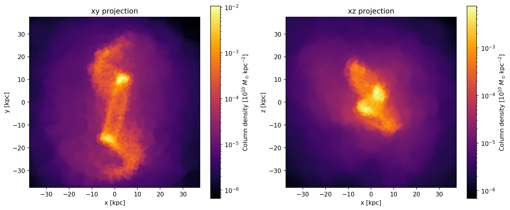
Plotting the result¶

Python

fig, axes = plt.subplots(1, 2, figsize=(12, 5))

vt.plot.plot_grid(
    image_xy,
    extent=[-L / 2, L / 2, -L / 2, L / 2],
    ax=axes[0], label="Column density",
)
axes[0].set_xlabel("x")
axes[0].set_ylabel("y")
axes[0].set_title("xy projection")

vt.plot.plot_grid(
    image_xz,
    extent=[-L / 2, L / 2, -L / 2, L / 2],
    ax=axes[1], label="Column density",
)
axes[1].set_xlabel("x")
axes[1].set_ylabel("z")
axes[1].set_title("xz projection")

Side-by-side xy and xz density projections

Projection planes¶

In Python, the proj parameter provides a shorthand for the six Cartesian projection planes: 'xy' (default), 'xz', 'yz', 'yx', 'zx', 'zy'. The center parameter is required for all planes except the default 'xy'.

In C++, you construct the ray grid manually and can orient it in any direction.