Volume Rendering¶

Volume rendering produces an RGB image by compositing color and opacity along each ray using emission-absorption integration. Unlike a density projection (which sums a quantity), volume rendering maps cell quantities through a transfer function to (R, G, B, alpha) and applies front-to-back compositing:

\[c(s) = \int_0^s c(s') \, \alpha(s') \, e^{-\tau(s')} \, ds', \qquad \tau(s) = \int_0^s \alpha(s') \, ds'\]

where \(\alpha\) is the absorption coefficient per unit length and \(\tau\) is the optical depth. The final color \(c(s)\) is an integral over the full ray length from 0 to s.

Note

Unlike simple integrals (Sum, Max, Min), the order of the ray start and end positions matters for volume rendering. The ray is composited front-to-back, so swapping start and end will produce a different image.

Defining a transfer function¶

The transfer function maps cell quantities to four values: red, green, blue, and absorption. You define this yourself. In the example below we use three physical channels – density (red), star-formation rate (green), and temperature (blue) – with density-driven opacity:

Python

import numpy as np

def lognorm(q, plo=1, phi=99):
    """Log-normalise positive array *q* to [0, 1]."""
    lq = np.log10(np.clip(q, q[q > 0].min(), None))
    lo, hi = np.percentile(lq, plo), np.percentile(lq, phi)
    return np.clip((lq - lo) / (hi - lo), 0, 1)

dens_norm = lognorm(rho)
R = 0.4 * dens_norm
G = np.where(sfr > 0, lognorm(np.where(sfr > 0, sfr, 1.0)), 0.0)

# Blue only for hot gas (T > 1.5e6 K), faded in dense regions
hot = np.clip((np.log10(np.maximum(T, 1.0)) - np.log10(1.5e6)) / 1.5, 0, 1)
B = 3.0 * hot * (1 - dens_norm) ** 2

# Opacity: dense gas or hot gas is visible
alpha = np.maximum(0.08 * dens_norm ** 4, 0.01 * hot ** 2)

fields_rgba = np.column_stack([R, G, B, alpha])

C++

#include <cmath>
#include <vector>
#include <algorithm>

// Build RGBA fields from density, SFR, and temperature.
// fields must have space for 4 * n doubles.
void transfer(const double* rho, const double* sfr,
              const double* T, size_t n, double* fields,
              double rho_lo, double rho_hi) {
    for (size_t i = 0; i < n; i++) {
        double d = std::clamp((std::log10(rho[i]) - rho_lo)
                              / (rho_hi - rho_lo), 0.0, 1.0);
        double hot = std::clamp((std::log10(std::max(T[i], 1.0))
                                 - std::log10(1.5e6)) / 1.5, 0.0, 1.0);
        double fade = (1 - d) * (1 - d);

        fields[i*4 + 0] = 0.4 * d;                      // R: density
        fields[i*4 + 1] = sfr[i] > 0 ? /* normalised SFR */ 0 : 0; // G: SFR
        fields[i*4 + 2] = 3.0 * hot * fade;             // B: temperature
        fields[i*4 + 3] = std::max(0.08*d*d*d*d, 0.01*hot*hot); // alpha
    }
}

Running the volume render¶

Python

import vortrace as vt

pc_vol = vt.ProjectionCloud(
    pos, fields_rgba, vol=vol,
    boundbox=[0, BoxSize, 0, BoxSize, 0, BoxSize],
)

image = pc_vol.grid_projection(
    extent, npix, bounds, center=None, reduction="volume"
)
# image.shape == (256, 256, 3) -- an RGB image

C++

#include <vortrace/vortrace.hpp>

// fields is a flat array with 4 values per particle: R, G, B, alpha
PointCloud cloud;
cloud.loadPoints(pos, npart, fields, npart, 4, subbox);
cloud.buildTree();

Projection proj(starts, ends, ngrid);
proj.makeProjection(cloud, ReductionMode::VolumeRender);

const auto& data = proj.getProjectionData();
// data has 3 values per ray (RGB): data[i * 3 + 0..2]

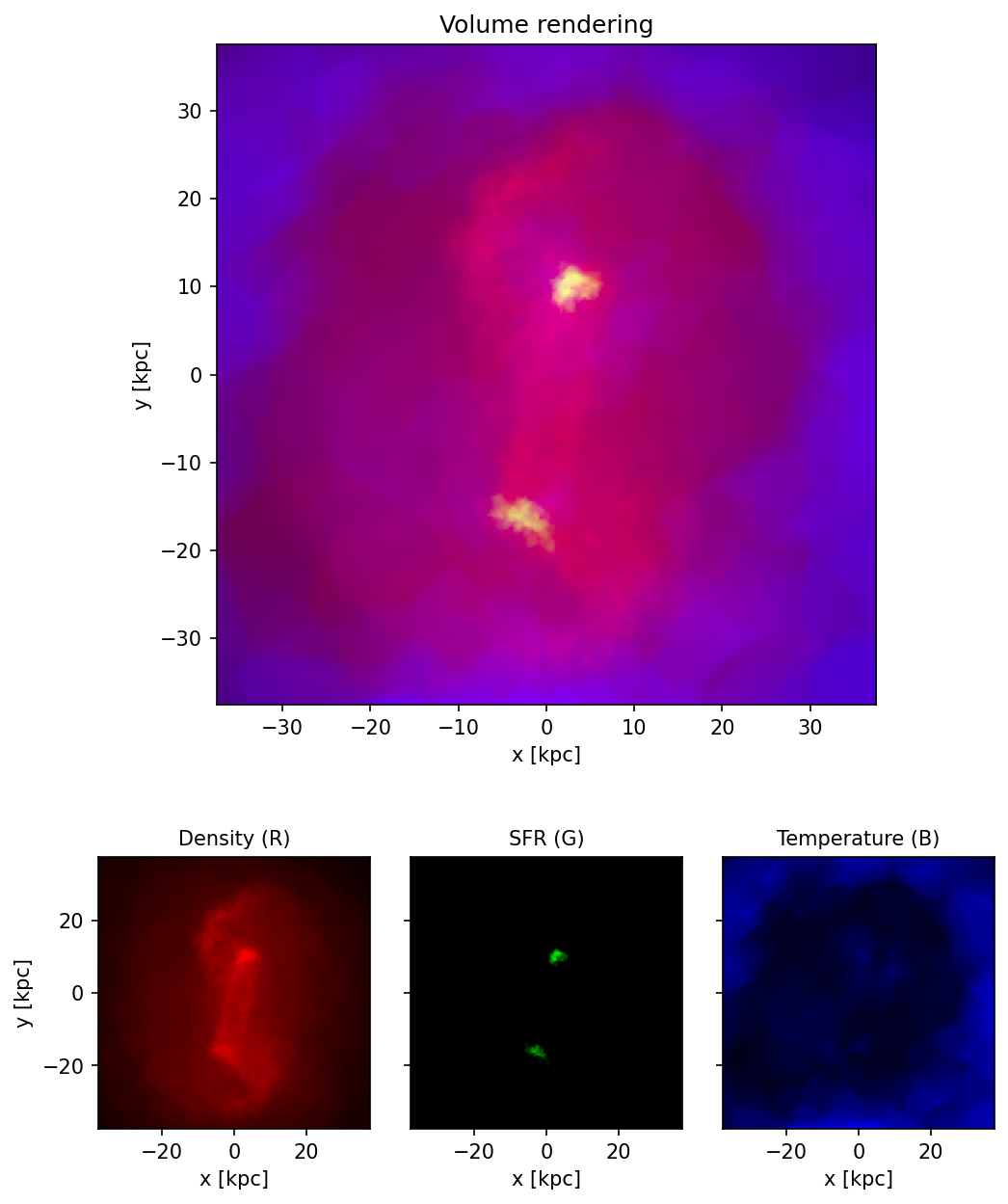
Displaying the result¶

The result is an RGB image. Red is tracing the total density. Green shows the regions with high star formation rate (centers of the galaxies). Blue shows the hot gas, which is mostly on the outskirts.

Python

import matplotlib.pyplot as plt

# Normalise each channel independently, then gamma-stretch
img = image.copy()
for c in range(3):
    mx = img[:, :, c].max()
    if mx > 0:
        img[:, :, c] /= mx
img = np.clip(img ** (1 / 2.0), 0, 1)  # gamma = 2

fig, ax = plt.subplots(figsize=(6, 6))
ax.imshow(np.swapaxes(img, 0, 1), origin="lower",
          extent=[-L / 2, L / 2, -L / 2, L / 2])
ax.set_xlabel("x [kpc]")
ax.set_ylabel("y [kpc]")

Volume rendering of a galaxy interaction

Note

Volume rendering requires exactly 4 input fields interpreted as (R, G, B, alpha). The output has 3 values per ray (RGB).